Graph Algorithm Parallelism
So far, we have seen pretty limited parallelism in our graph algorithms:
- BFS: Span=$O(d \lg^2 n)$, where $d$ is the diameter of graph
- So, serial in the worst case.
- DFS, Dijkstra, Prim, Kruskal: serial
- Bellman-Ford: Update shortest paths to each node in parallel, span = $O(|V| \lg |V|)$
- Johnson: can run Dijkstra in parallel for each source, span=$O(|E| \lg |V|)$
Is there any way to expose more parellelism?
Divide and conquer on graphs
What would a divide and conquer algorithm look like for graphs?
Could we partition the graph and combine solutions to each partition?
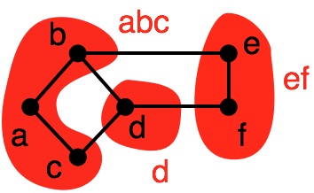
Want nearly equal-sized partitions -- this is hard to compute!
The edges between partitions will make it difficult to solve subproblems independently.
Contraction
Recall contraction, which we used to implement scan:
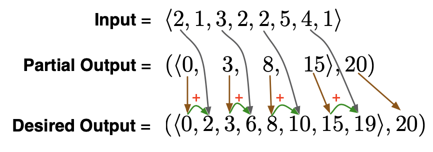
- Reduce problem size by a constant factor (e.g., half as large). (contraction)
- Solve this smaller problem.
- Expand solution to solve the larger problem. (expansion)
We'll develop contraction algorithms to achieve better parallelism in graph algorithms.
Graph partitions
How can we partition a graph?
Recall the notion of graph cut:
A graph cut of a graph $(G,V)$ is a partitioning of vertices $V_1 \subset V$, $V_2 = V - V_1$.
Each vertex set $V_i \subset V$ defines a vertex-induced subgraph consisting of edges where both endpoints are in $V_i$.
For example:
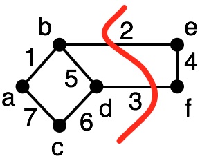
In this partition, we have:
- $G_1 = (V_1, E_1)~~~~V_1=\{a,b,c,d\}, E_1 = \{(a,b), (a,c), (c,d), (b,d)\}$
- $G_2 = (V_2, E_2)~~~~V_2=\{e,f\}, E_2 = \{(e,f)\}$
The cut edges are those that join the two subgraphs, e.g., $\{(b,e), (d,f)\}$.
Graph partition
a collection of graphs $\{G_1 = (V_1, E_1), \ldots, G_{k} = (V_{k}, E_{k})\}$ such that
- $\{V_1, \ldots, V_{k}\}$ is a set partition of $V$.
- $\{G_1, \ldots, G_{k}\}$ are vertex-induced subgraphs of $G$ with respect to $\{V_1, \ldots, V_{k}\}$.
We refer to each subgraph $G_i$ as a block or part of $G$.
For a given partition, we have two types of edges in $E$:
- cut edges: an edge $(v_1,v_2)$ such that $v_1 \in V_i$, $v_2 \in V_j$ and $V_i \ne V_j$
- internal edges: an edge $(v_1,v_2)$ such that $v_1 \in V_i$, $v_2 \in V_j$ and $V_i = V_j$
Graph Contraction: Intuition
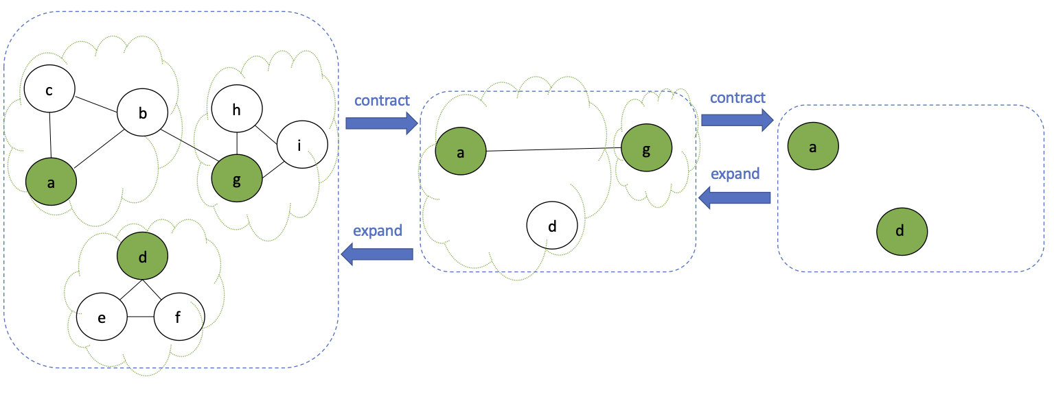

contract step:
- partition $G$ into subgraphs $\{G_1 \ldots G_k\}$
- Assign one vertex of each subgraph as a super vertex
- e.g., $a$, $d$, $g$ are super vertices of first contraction step
- drop internal edges
- reroute internal edges to connect super vertices
- e.g., $(a,g)$ is added in first contraction step because $(b,g)$ exists in first graph

recursive step:
- Solve problem for each subgraph in the partition
- base case: stop when no more edges in the graph

expansion step:
- combine solutions to subgraphs to compute result for original input graph
How should we choose partitions?
We want partitions that:
- respect the connectivity of the original graph.
- i.e., vertices in the same partition should be connected
- shrinks the graph by a constant fraction (geometric decrease)
- to ensure a logarithmic span ($\lg n$ rounds of contraction)
We'll look at different ways of partitioning in a moment. For now, let's look at an example of how contraction works to solve a specific problem without worrying too much about the details of the partitioning.
General contraction
# graph contraction
# we still need to specify partition_graph_f!

def contract_graph(vertices, edges, partition_graph_f):
    if len(edges) == 0:
        return vertices, edges
    else:
        # partition the graph
        # vertex_map is a dict from vertex->super_vertex
        # e.g., {'a': 'a', 'b': 'a', 'c': 'a'...} in above example
        new_vertices, vertex_map = partition_graph_f(vertices, edges)
        # keep only cut eges
        new_edges = set([(vertex_map(e[0]), vertex_map(e[1]))
                          for e in edges if vertex_map(e[0]) != vertex_map(e[1])])
        return contract_graph(new_vertices, new_edges, partition_graph_f)

vertices = set(['a', 'b', 'c', 'd', 'e', 'f', 'g', 'h', 'i'])
edges = set([('a', 'b'), ('a', 'c'), ('b', 'c'), ('b', 'g'),
             ('d', 'e'), ('d', 'f'), ('e', 'f'),
             ('h', 'i'), ('i', 'g'), ('h', 'g')])

contract_graph(vertices, edges, partition_graph_f)
Contraction example: Number of connected components
Recall in recitation, we have computed the number of connected components in a graph.
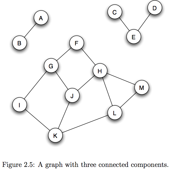
How did we do this? What was the worst-case span of our approach?
Connected components via contraction
Now let's think how we might do this with graph contraction.

What does the connectivity in the contracted graph tell us about the connectivity in the original graph?

Since $a$, $b$, $c$ are placed in the same partition, we know they are connected.
Since $a$ and $g$ are connected in the second graph, then every node in the $g$ partition is reachable from every node in the $a$ partition.
Similarly, since $d$ is not connected to $a$ or $g$, then we know that no node in the $d$ partition is reachable from any node in either the $a$ or $g$ partition.
What does the final contracted graph tell us about the number of connected components?
Num components, contraction style
# we still need to specify partition_graph_f!

def num_components(vertices, edges, partition_graph_f):
    if len(edges) == 0:
        # base case: return the number of super vertices in the final partition
        return len(vertices)
    else:
        new_vertices, vertex_map = partition_graph_f(vertices, edges)
        # keep only cut eges
        # can use filter here to do in parallel: O(log|E|) span
        new_edges = set([(vertex_map[e[0]], vertex_map[e[1]])
                          for e in edges if vertex_map[e[0]] != vertex_map[e[1]]])
        return num_components(new_vertices, new_edges, partition_graph_f)
vertices = set(['a', 'b', 'c', 'd', 'e', 'f', 'g', 'h', 'i'])
edges = set([('a', 'b'), ('a', 'c'), ('b', 'c'), ('b', 'g'),
             ('d', 'e'), ('d', 'f'), ('e', 'f'),
             ('h', 'i'), ('i', 'g'), ('h', 'g')])
num_components(vertices, edges, partition_graph_f)
While we have not yet specified partition_graph_f, let's assume it
- returns a graph of size $|V|/2$
- has $O(\lg |V|)$ span.
What is the recurrence for the full algorithm to compute num_components?
$S(|V|) = S\left(\frac{|V|}{2}\right) + \lg (|V|)$
which evaluates to?
$O(\lg^2 |V|)$
This is much better than the span for our BFS/DFS implementations of num_components.
$O(|V| + |E|)$
Take-aways?
To get this level of parallelism, we need a way of partitioning a graph that has low span and reduces the number of vertices by a contant (geometric) factor each round.
- the low span requirement means we can't do anything that requires a graph search
This is nice because:
- We reduce |V| in half (at least in this example)
- It maintains the connectivity of the original graph
- It seems somewhat easy to compute.
Here's a simple way to find an edge partition: Randomly pick half the edges in the graph
What can go wrong with this approach?
We don't want to have the same node in two partitions.
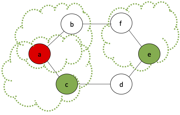
What is a greedy algorithm to avoid this case?
Initialize an empty edge set M

Iterate over each edge e in the graph:
    If the vertices in e don't appear in M, add it to M
What is the span of this algorithm?
$O(|E|)$ -- it is sequential, every choice depends on previous choices.
Can we come up with a parallel version of this idea? Hint: use randomness
Parallel Edge Partition
We can randomly select edges, contigent on certain conditions.
- Flip a coin for each edge, in parallel, assigning $H$ or $T$ to each edge
- Run a
filteron all the results, selecting those edges $e$ where:- $e$ has $H$
- all edges incident on $e$ are $T$
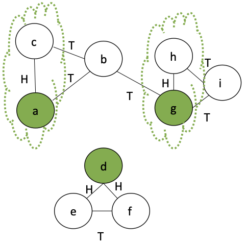

Here, we make partitions for two edges: $\{a,c\}, \{g,h\}$
The rest are put in their own singleton partitions: $\{b\}, \{d\}, \{e\}, \{f\}, \{i\}$
Implementation
def edge_contract(vertices, edges):
    # sample each edge with 50% chance
    sampled_edges = [e for e in edges if random.choice([True, False])]
    #print('%d/%d sampled edges' % (len(sampled_edges), len(edges)))
    #print(sorted(sampled_edges))
    # count how often each vertex appears in the sampled edges.
    # could do this in parallel (map-reduce) in O(log |V|) span
    vertex_counts = Counter()
    for p in sampled_edges:
        vertex_counts.update(p)
    #print('\nvertex counts in sampled edges:', vertex_counts.items())

    # now, do a filter to get those edges where both vertices
    # appear only once in sampled_edges
    valid_edges = [e for e in sampled_edges if vertex_counts[e[0]] == 1 and vertex_counts[e[1]]==1]
    #print('\nkeeping these valid edges:', valid_edges)

    # make partitions
    vertex_map = dict()
    for e in valid_edges:
        vertex_map[e[0]] = e[1]
    # put all the rest in a singleton partition
    for v in vertices:
        if v not in vertex_map:
            vertex_map[v] = v
    return set(vertex_map.values()), vertex_map
def num_components(vertices, edges, partition_graph_f):
    if len(edges) == 0:
        # base case: return the number of super vertices in the final partition
        return len(vertices)
    else:
        new_vertices, vertex_map = partition_graph_f(vertices, edges)
        # keep only cut eges
        # can use filter here to do in parallel: O(log|E|) span
        new_edges = set([(vertex_map[e[0]], vertex_map[e[1]])
                          for e in edges if vertex_map[e[0]] != vertex_map[e[1]]])
        return num_components(new_vertices, new_edges, partition_graph_f)

vertices = set(['a', 'b', 'c', 'd', 'e', 'f', 'g', 'h', 'i'])
edges = set([('a', 'b'), ('a', 'c'), ('b', 'c'), ('b', 'g'),
             ('d', 'e'), ('d', 'f'), ('e', 'f'),
             ('h', 'i'), ('i', 'g'), ('h', 'g')])
num_components(vertices, edges, edge_contract)
2
By construction, we know that this will be a valid partitioning.
But, will it make the graph small enough fast enough?
Consider a cycle graph, where each vertex has exactly two neighbors:
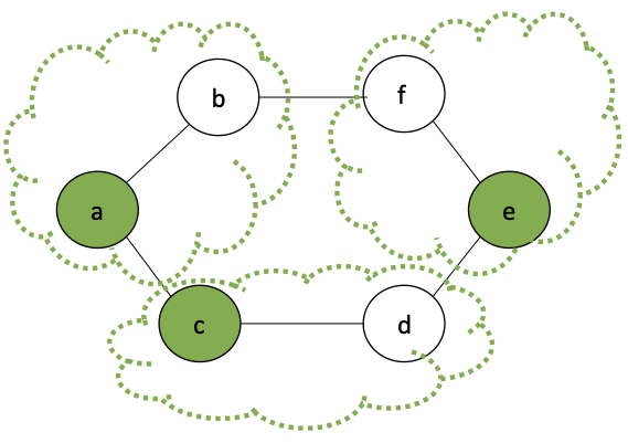
What is the probability that a given edge $e$ will be selected for a partition?
This is the probability that: it is $H$, and it's two neighboring edges are $T$
Will we contract at a constant fraction of the graph size?
So, if there are $|E|$ edges, and each has probability of $\frac{1}{8}$ of being selected, then what is the expected number of edges selected at each round?
Since $|V| = |E|$ in a cycle graph, and since we remove 1 vertex for each edge partition we select, we will reduce the number of vertices by $\frac{1}{8}$ at each round, in expectation.
Thus, the recurrence:
But, we have assumed a cycle graph. What would be a graph structure where edge contraction performs poorly? (i.e., doesn't remove enough edges)?
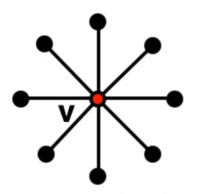
Next time: Star Graphs!