Agenda
- Introduce spanning trees and Prim's Algorithm
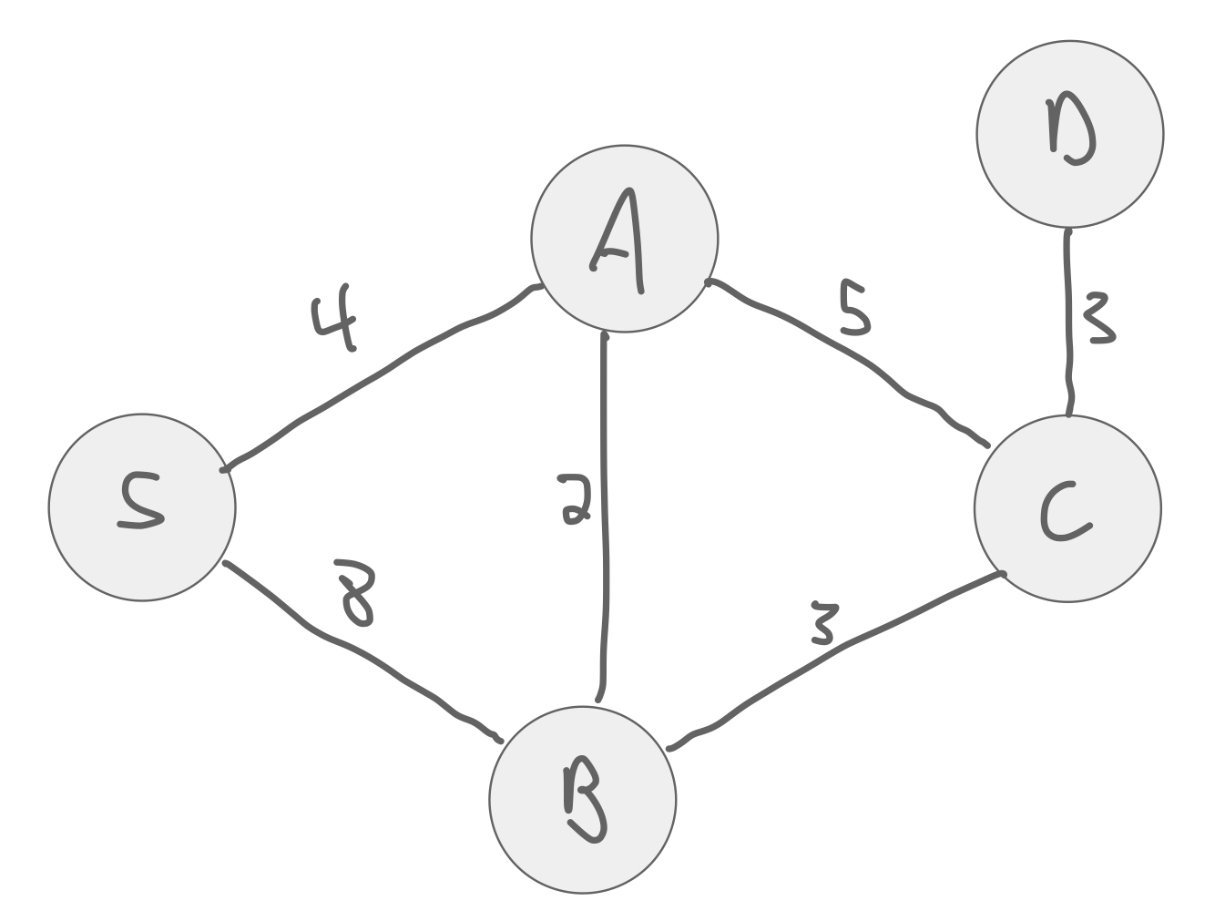
Recall breadth-first search. Starting from vertex $s$, what order will the vertices be visited in this graph?
Because we avoid revisiting nodes, we can view the edges we visit as a tree.
for n in graph[node]:
    if n not in visited:
        frontier.append(n)
This tree includes all vertices. We call this a spanning tree.
For a connected undirected graph $G = (V,E)$, a spanning tree is a tree $T = (V,E')$ with $E' \subseteq E$
Finding spanning trees
What are some algorithms we can use to find a spanning tree of a graph?
BFS and DFS can both be used.
They have the work, though BFS can have better span: $O(d \lg^2 n)$, where $d$ is the diameter of the graph.
The diameter of a graph is the length of the shortest path between the most distant vertices.
We refer to the weight of a tree $T$ with edges $E(T)$ as:
$$w(T) = \sum_{e \in E(T)} w(e)$$Is there a smaller tree in this graph?
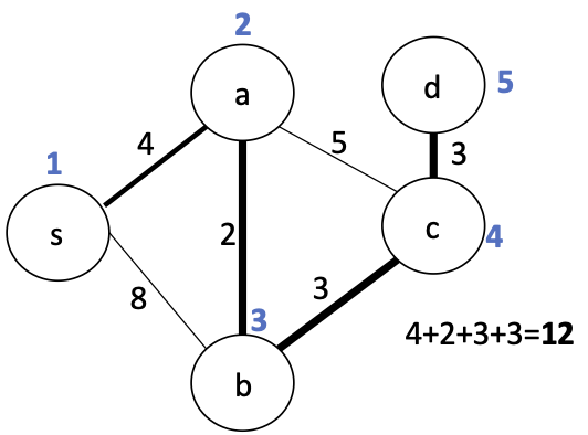
This is called the minimum spanning tree (MST) of the graph.
Applications of MSTs
What are some applications where we might want to find the MST?
- Power grid
- minimize cost
- Transportation networks
- build bridges between towns
- minimize building cost
- Computer networks
- Cycle free routing
History of MSTs
Otakar Borůvka first identified and solved this problem in 1926 to build an efficient electricity network in (present day) Czech Republic.
"Soon after the end of World War I, at the beginning of the 1920s, the Electric Power Company of Western Moravia, Brno, was engaged in rural electrification of Southern Moravia. In the framework of my friendly relations with some of their employees, I was asked to solve, from a mathematical standpoint, the question of the most economical construction of an electric power network. I succeeded in finding a construction -- as it would be expressed today -- of a maximal connected subgraph of minimum length, which I published in 1926 (i.e., at a time when the theory of graphs did not exist)."
Considering the MST problem
What is the brute-force approach to find the MST?
As usual, we have an exponential search space.
There are an exponential number of possible spanning trees to consider.
Can we just select edges in increasing order of weight?
Edge replacement lemma
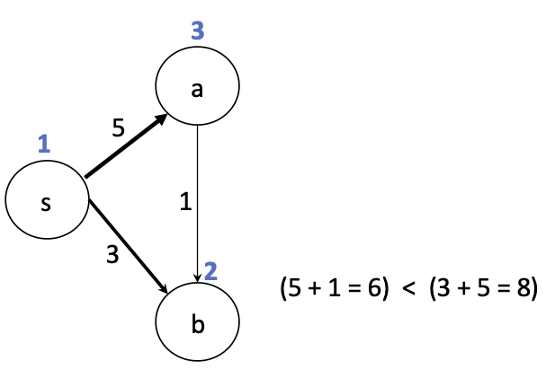
Let's think about how we can modify one spanning tree to get another one. Maybe we can iteratively refine a tree to reduce its weight...
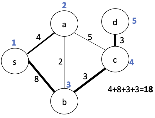
Replacing $(s,b)$ with $(a,b)$ reduces the cost:
Edge Replacement
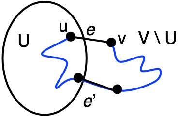
- Consider a spanning tree $T$ containing an edge $e=(a,b)$ on the path from $u$ to $v$.
- Consider another edge $e'=(u,v)$ that is not in $T$.
- What happens if we remove $e$ from $T$ and insert $e'$
- Will it still be a tree?
Yes:
- We can re-route the path from $u$ to $v$ to use $e'$ instead of $e$.
- Thus, the new tree remains connected and acyclic.
We will combine this idea with shortest path algorithms to explore several algorithms to find the MST.
- As in shortest path algorithms, we need a $visited$ and $frontier$ sets.
- We need to decide which edge to add to the tree to minimize the weight.
Graph cut
We can view the $visited$ and $frontier$ sets as defining a graph cut.
A graph cut of a graph $(G,V)$ is a partitioning of vertices $V_1 \subset V$, $V_2 = V - V_1$.
Each vertex set $V_i \subset V$ defines a vertex-induced subgraph consisting of edges where both endpoints are in $V_i$.
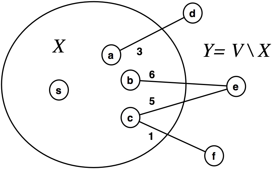
For example:
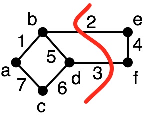
In this partition, we have:
- $G_1 = (V_1, E_1)~~~~V_1=\{a,b,c,d\}, E_1 = \{(a,b), (a,c), (c,d), (b,d)\}$
- $G_2 = (V_2, E_2)~~~~V_2=\{e,f\}, E_2 = \{(e,f)\}$
The cut edges are those that join the two subgraphs, e.g., $\{(b,e), (d,f)\}$.
Light-edge property
Let $G = (V,E,w)$ be a connected undirected, weighted graph with distinct edge weights.
For any cut of $G$, the minimum weight edge that crosses the cut is contained in the minimum spanning tree of $G$.
Theorem: For any cut of $G$, the minimum weight edge that crosses the cut is contained in the minimum spanning tree of $G$.
Proof by Contradiction: Assume that the lightest edge $e = \{u,v\}$ is not in the MST.
Then, there must be some other path connecting $u$ to $v$ that goes through some other edge $e'$.
By assumption, $e'$ must be heavier that $e$.
But, by the Edge Replacement Lemma, we know that we can swap $e'$ for $e$ and still having a spanning tree, one that will be lighter. This is a contradiction. $\blacksquare$
How can we use the light-edge property to find the MST using priority search?
Prim's Algorithm
Iteratively build a MST by performing priority-first search on $G$ starting from an arbitrary vertex $s$.
To select the next edge to expand the frontier $X$, use priority:
- $p(v) = \min_{x \in X, v \in Y} w(x,v)$
- Add the chosen edge $(u,v)$ to the tree.
- Edge $(c, f)$ has minimum weight across the cut $(X,Y)$.
- So, we visit $f$ by adding $(c, f)$ to the tree and all of $f$'s neighbors to the frontier
This sounds very similar to Dijkstra's algorithm. What's the difference?
from heapq import heappush, heappop

def dijkstra(graph, source):
    def dijkstra_helper(visited, frontier):
        if len(frontier) == 0:
            return visited
        else:
            distance, node = heappop(frontier)
            if node in visited:
                return dijkstra_helper(visited, frontier)
            else:
                print('visiting', node)
                visited[node] = distance
                for neighbor, weight in graph[node]:
                    heappush(frontier, (distance + weight, neighbor))
                return dijkstra_helper(visited, frontier)

    frontier = []
    heappush(frontier, (0, source))
    visited = dict()  # store the final shortest paths for each node.
    return dijkstra_helper(visited, frontier)
def prim(graph):
    def prim_helper(visited, frontier, tree):
        if len(frontier) == 0:
            return tree
        else:
            weight, node, parent = heappop(frontier)
            if node in visited:
                return prim_helper(visited, frontier, tree)
            else:
                print('visiting', node)
                # record this edge in the tree
                tree.add((weight, node, parent))
                visited.add(node)
                for neighbor, w in graph[node]:
                    heappush(frontier, (w, neighbor, node))
                    # compare with dijkstra:
                    # heappush(frontier, (distance + weight, neighbor))

                return prim_helper(visited, frontier, tree)

    # pick first node as source arbitrarily
    source = list(graph.keys())[0]
    frontier = []
    heappush(frontier, (0, source, source))
    visited = set()  # store the visited nodes (don't need distance anymore)
    tree = set()
    prim_helper(visited, frontier, tree)
    return tree
Work of Prim's Algorithm
This does identical work to Dijkstra, so $O(|E| \log |V|)$
Can we just pick an arbitrary source node? Why or why not?
Directed Graphs?
What about directed graphs? Will this work?
No - if source node is not connected to all other nodes.
Even if it is, we may have a suboptimal solution: