Recall that Dijkstra's algorithm assumed positive edge weights. Why?

Dijkstra's property
For any partitioning of vertices $V$ into $X$ and $Y = V \setminus X$ with $s \in X$:
If $p(v,x) = \min_{x \in X} (\delta_G(s,x) + w(x,v))$, then
$$\min_{y \in Y} p(y) = \min_{y \in Y} \delta_G(s, y)$$What goes wrong in this example?
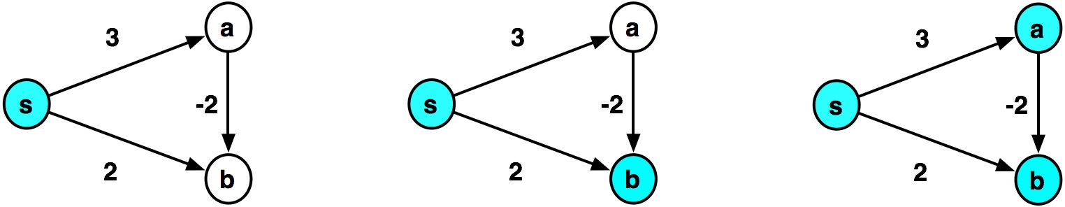
- At the second step, Dijkstra assigns $\delta(s,b)\leftarrow 2$
- When $a$ is visited in the third step, $b$ would be added to the heap with distance $1$.
- But, when $b$ is popped off the heap the second time, it is ignored, because of:
if node in visited:
              # Already visited, so ignore this longer path
              return dijkstra_helper(visited, frontier)
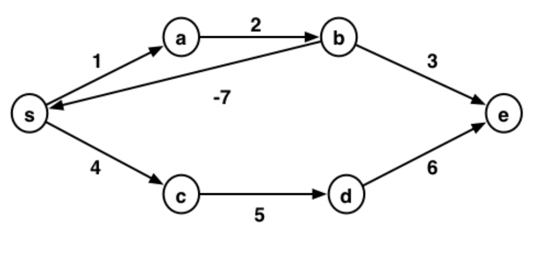
With negative edge weights, paths can get shorter as we add edges!
Why would we ever have a graph with negative edge weights?
- finance: cost versus profit
- chemistry: attractive vs repulsion
Dealing with negative edge weights
Since paths can get shorter as we add edges, we'll modify Dijkstra to instead keep track of both the weight and the number of edges in a path.
$\delta^k(u,v)$: weight of shortest path from $u$ to $v$ considering paths with at most $k$ edges.
- If no such path exists, $\delta^k(u,v)=\infty$
Consider negative cycles: sum of weights in a cycle is less than 0
If there are no negative cycles:
- then the shortest path between any two nodes contains no cycles
- thus, the shortest path has at most $|V|-1$ edges
- compute $\delta^k(u,v)$ from $k=1$ to $k=|V|-1$
If there are negative cycles:
- then the shortest path has weight $-\infty$
- must detect such cycles while computing $\delta^k(u,v)$
Computing $\delta^{k+1}(u,v)$
As usual, we will assume we have recursively computed $\delta^k(s,v)$. To extend this to compute $\delta^{k+1}(s,v)$:
$$ \begin{align} \delta^{k+1}(s, v) = \min&(\delta^{k}(s, v),\\ &\min_{x \in N^-(v)} (\delta^{k}(s, x) + w(x,v)) \end{align} $$where $N^-(v)$ are the in-neighbors of $v$
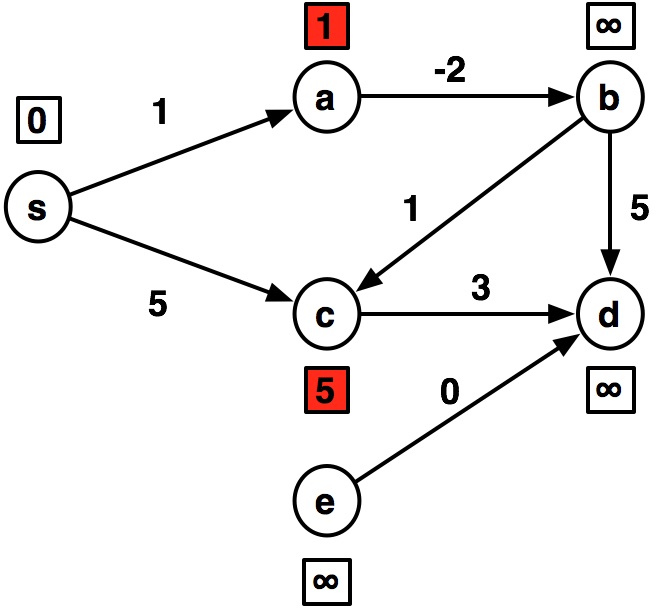
Consider this graph, where we have already computed the shortest paths from the source $s$ to vertices using $k$ or fewer edges.
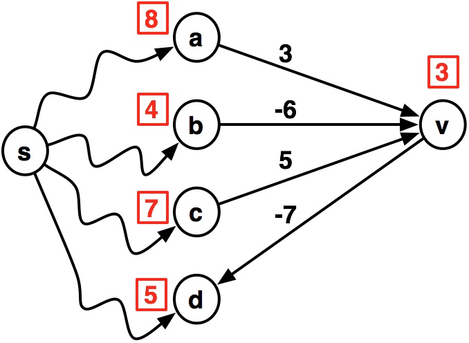
- Each vertex $u$ is labeled with $\delta^k(s,u)$, its $k$-distance from $s$
- Then, the shortest path to $v$ using at most $k+1$ edges is
Bellman-Ford Algorithm
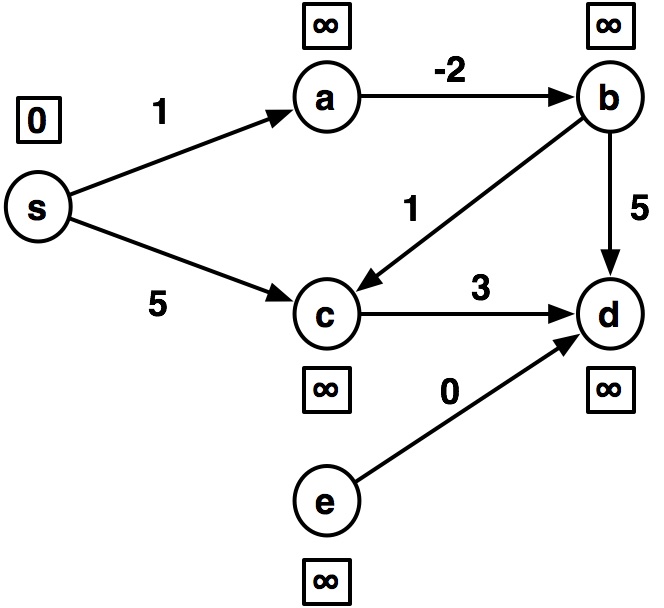
- Initialize: $\delta^0(s,s)=0$ and $\delta^0(s,v)=\infty$ $\forall ~ v \ne s$
- Iterate: Compute $\delta^{k+1}(s,v)$ $\forall v$ as above, using $\delta^{k}(s,v)$ $\forall v$
- We can compute this in parallel for all $v$
When to stop?
Stop when the values converge, that is, when the next iteration makes no updates:
When $\delta^{k+1}(s,v)=\delta^{k}(s,v)$ $~\forall ~~ v$
but: if there are negative cycles, this may never be true.
So, we can instead stop after $|V|$ iterations.
- if we haven't converged at that point, then there must be a negative cycle
Let's look at code and output on this example:
import math

def bellmanford(graph, source):
    def bellmanford_helper(distances, k):
        if k == len(graph): # negative cycle
            return -math.inf
        else:
            # compute new distances
            new_distances = compute_distances(graph, distances)

            # check if distances have converged
            if converged(distances, new_distances):
                return distances
            else:
                return bellmanford_helper(new_distances, k+1)

    # initialize
    distances = dict()
    for v in graph:
        if v == source:
            distances[v] = 0
        else:
            distances[v] = math.inf
    return bellmanford_helper(distances, 0)
def compute_distances(graph, distances):
    print("\n----")
    new_distances = {}
    for v, in_neighbors in graph.items(): # this loop can be done in parallel
        # compute all possible distances from s->v
        v_distances = [distances[v]]
        for in_neighbor, weight in in_neighbors:
            v_distances.append(distances[in_neighbor] + weight)
        new_distances[v] = min(v_distances)
        print("{}:{}  ".format(v, new_distances[v]), end='')
    return new_distances

def converged(old_distances, new_distances):
    return old_distances == new_distances
# instead, represent in-neighbors for each node, for constant lookup
graph = {
            's': {},
            'a': {('s', 1)},# ('c', 0)},
            'b': {('a', -2)},
            'c': {('s', 5), ('b', 1)},
            'd': {('b', 5), ('c', 3), ('e', 0)},
            'e': {},
        }
# original representation: map from node to out-neighbors
# graph = {
#             's': {('a', 1), ('c', 5)},
#             'a': {('b', -2)},
#             'b': {('c', 1), ('d', 5)},
#             'c': {('d', 3)},
#             'd': {},
#             'e': {('d', 0)}
#         }
bellmanford(graph, 's')
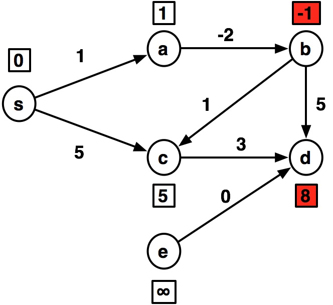
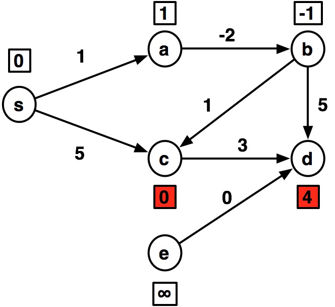
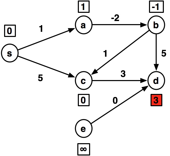
----
s:0  a:1  b:inf  c:5  d:inf  e:inf
----
s:0  a:1  b:-1  c:5  d:8  e:inf
----
s:0  a:1  b:-1  c:0  d:4  e:inf
----
s:0  a:1  b:-1  c:0  d:3  e:inf
----
s:0  a:1  b:-1  c:0  d:3  e:inf
{'s': 0, 'a': 1, 'b': -1, 'c': 0, 'd': 3, 'e': inf}
graph2 = {
            's': {},
            'a': {('s', 1), ('c', -1)}, # make a negative cycle a->b->c->a, -2
            'b': {('a', -2)},
            'c': {('s', 5), ('b', 1)},
            'd': {('b', 5), ('c', 3)},
            'e': {},
        }
bellmanford(graph2, 's')
----
s:0  a:1  b:inf  c:5  d:inf  e:inf
----
s:0  a:1  b:-1  c:5  d:8  e:inf
----
s:0  a:1  b:-1  c:0  d:4  e:inf
----
s:0  a:-1  b:-1  c:0  d:3  e:inf
----
s:0  a:-1  b:-3  c:0  d:3  e:inf
----
s:0  a:-1  b:-3  c:-2  d:2  e:inf
-inf
Cost of Bellman-Ford
def compute_distances(graph, distances):
    new_distances = {}
    for v, in_neighbors in graph.items(): # this loop can be done in parallel
        v_distances = [distances[v]]
        for in_neighbor, weight in in_neighbors:
            v_distances.append(distances[in_neighbor] + weight)
        new_distances[v] = min(v_distances)
    return new_distances
Work
- For each vertex, we loop through all of its in-neighbors.
- We then take the minimum over its in-neighbors
- Thus, we will visit each edge in the graph once in each iteration of the algorithm ($|E|$)
- There are at most $|V|$ iterations of the algorithm, to the total work for
compute_distancesis $O(|V| \cdot |E|)$.
def compute_distances(graph, distances):
    new_distances = {}
    for v, in_neighbors in graph.items(): # this loop can be done in parallel
        v_distances = [distances[v]]
        for in_neighbor, weight in in_neighbors: # Can be done in O(1) span
            v_distances.append(distances[in_neighbor] + weight)
        new_distances[v] = min(v_distances) # Can be done in O(lg n) span
    return new_distances
Span
- Because we can do the outer loop in parallel, we must consider the maximum span of any vertex $v$.
- In the worst case, $v$ can have $|V|-1$ in-neighbors. The
minoperation will then take $O(\lg |V|)$ span, assuming we usereduceto implement it. - Thus, each iteration has $O(\lg |V|)$ span, and we have at worst $|V|$ iterations, run sequentially, resulting in total span of $O(|V| \lg |V|)$.
What about the work to check if we have converged?
def converged(old_distances, new_distances):
    return old_distances == new_distances
Under the hood:
def converged(old_distances, new_distances):
    for k in old_distances:
        if old_distances[k] != new_distances[k]:
            return False
    return True
This is $O(|V|)$
But, if we were more clever, we could include this check inside the compute_distances function, just before assigning the new_distances value.
...
min_v = min(v_distances)
if min_v != new_distances[v]:
    converged=False
new_distances[v] = min(v_distances)
...
so, we don't incur any additional cost for this check.
Final work/span of Bellman-Ford
Work: $O(|V| \cdot |E|)$
Span: $O(|V| \lg |V|)$
compare with:
Dijkstra:
$~~~$ Work $O(|E|\log |V|)$
$~~~$ Span $O(|E|\log |V|)$
BFS:
$~~~$ Work $O(|E|+ |V|)$
$~~~$ Span $O(|E| + |V|)$
So, we can see we pay significant costs going from unweighted $\rightarrow$ weighted-positive $\rightarrow$ weighted-negative graphs.
- Although, consider the difference in span between Dijkstra and Bellman-Ford
Bellman-Ford is used in network routing:

- Each router has a routing table containing the shortest path from source to destination
- Edge weights account for latency between routers.
- But, no router has perfect knowledge of the network.
- Routers exchange information in a peer-to-peer fashion to update routing tables.
- But wait, there can't be a negative weight in this graph! (no "negative latency").
- So, why use Bellman-Ford instead of Dijkstra?
- Bellman-Ford is naturally a distributed/concurrent algorithm -- each node updates its shortest paths and exchanges with neighbors.
- Dijkstra requires each node to have perfect knowledge of the network, in order to make the optimal, greedy step at each iteration.