CMPS 2200

Introduction to Algorithms

Shortest Paths

Generalizing DFS and BFS search

We've now seen two types of search that are conceptually very similar.

dfs_stack:

• node = frontier.pop()

bfs_serial:

• node = frontier.popleft()

Can we generalize these?

from collections import deque

def generic_search(graph, source, get_next_node_fn):
    def generic_search_helper(visited, frontier):
        if len(frontier) == 0:
            return visited
        else:
            ## pick a node
            node = get_next_node_fn(frontier)
            print('visiting', node)
            visited.add(node)
            frontier.extend(filter(lambda n: n not in visited, graph[node]))
            return generic_search_helper(visited, frontier)
        
    frontier = deque()
    frontier.append(source)
    visited = set()
    return generic_search_helper(visited, frontier)

def bfs_fn(frontier):
    return frontier.popleft()

def dfs_fn(frontier):
    return frontier.pop()

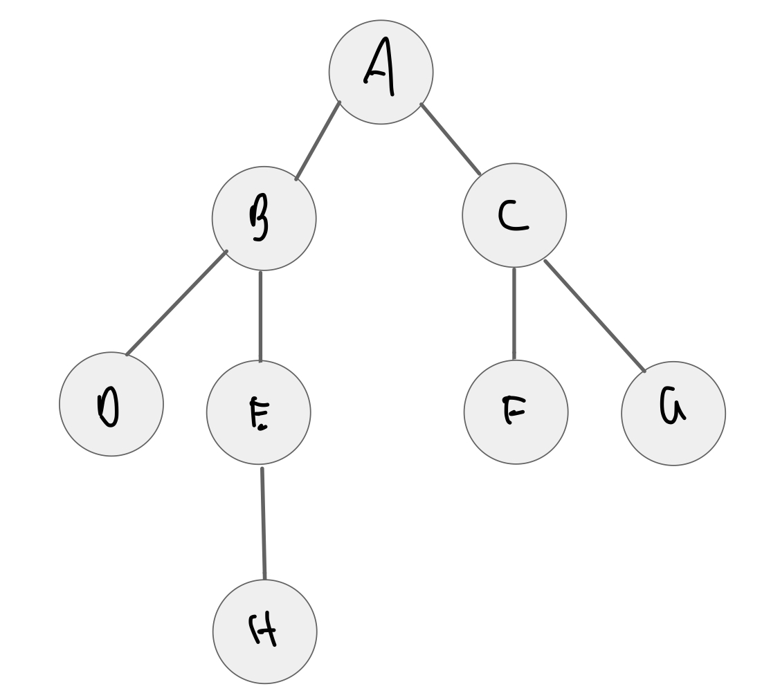
generic_search(graph, 'A', bfs_fn)

visiting A
visiting C
visiting B
visiting F
visiting G
visiting D
visiting E
visiting H

{'A', 'B', 'C', 'D', 'E', 'F', 'G', 'H'}

generic_search(graph, 'A', dfs_fn)

visiting A
visiting B
visiting E
visiting H
visiting D
visiting C
visiting F
visiting G

{'A', 'B', 'C', 'D', 'E', 'F', 'G', 'H'}

Priority First Search

We could use the get_next_node_fn as a way to pick the highest priority node to visit at each iteration.

E.g., consider a Web crawler that prioritizes which pages to visit first

• more interesting pages
• pages that update more frequently

We'll see several algorithms that are instances of priority first search.

Weighted graphs

Up to now we have focused on unweighted graphs.

For many problems, we need to associate real-valued weights to each edge.

E.g., a graph where nodes are cities and edges represent the distance between them.

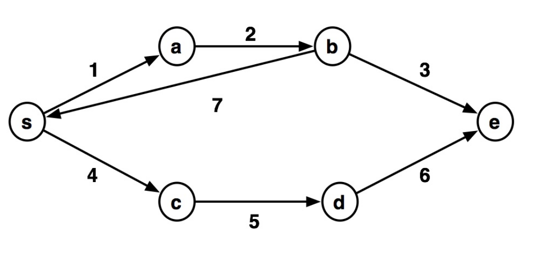
The weight of a path in the graph is the sum of the weights of the edges along that path.

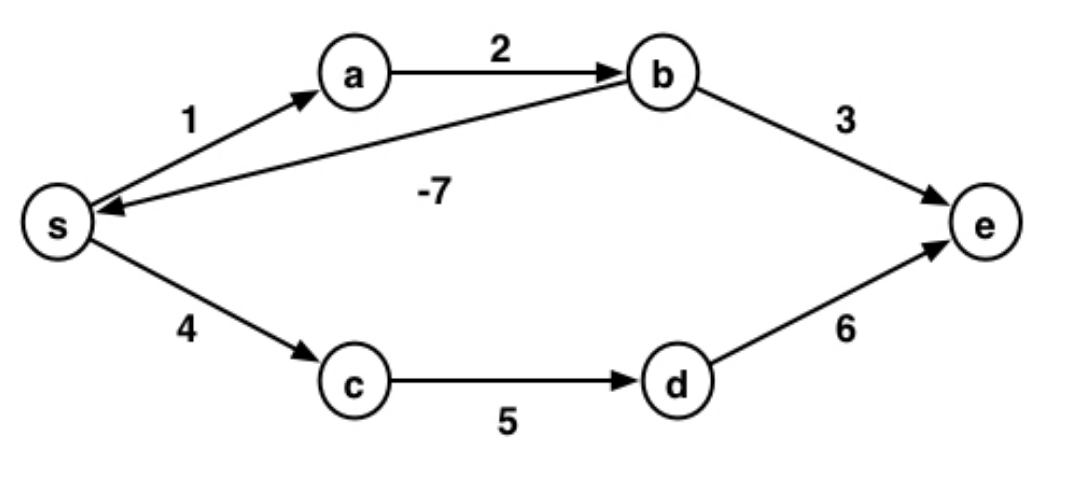
The shortest weighted path (or just shortest path) between s and e is the one with minimal weight.

What is the shortest path from s to e?

Use BFS to solve shortest path problem?

We saw that we can use BFS to get the distance from the source to each node.

Can we use BFS to solve the shortest path problem for weighted graphs?

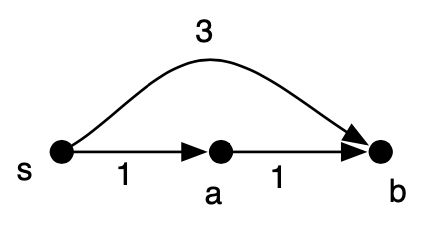
BFS will:

• visit b
• visit a
• but, will not traverse the path from a to b, since it doesn't visit a node more than once

Thus, BFS will not discover that the shortest path from $s$ to $b$ is $s \rightarrow a \rightarrow b$.

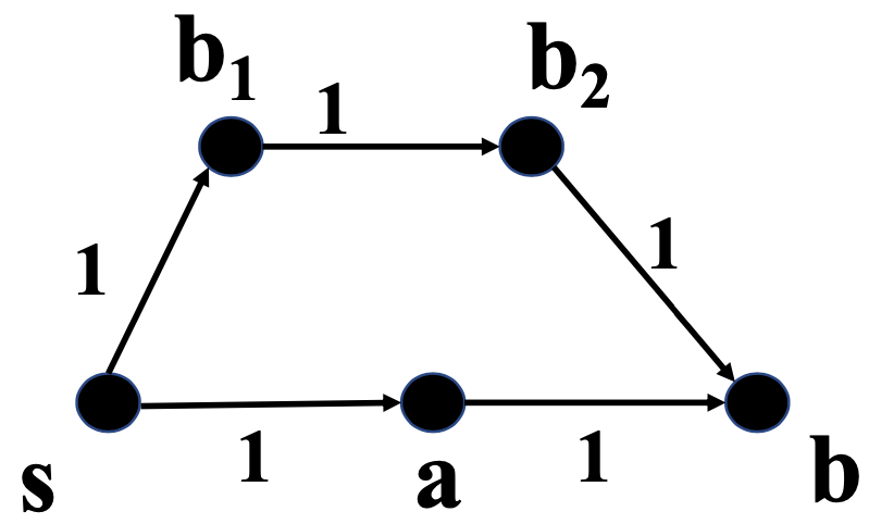
How could we modify the graph so we can use BFS to find the shortest path?

Consider another example:

What is the shortest path from $s$ to $e$?

Infinite loop in the cycle $s \rightarrow a \rightarrow b \rightarrow a$, so shortest path is $-\infty$

SSSP: Single-Source Shortest Path

Given a weighted graph $G=(V,E,w)$ and a source vertex $s$, the single-source shortest path (SSSP) problem is to find a shortest weighted path from $s$ to every other vertex in $V$.

What would be a brute-force solution to this problem?

Is there anything we could reuse to improve the brute-force solution?

Consider this figure:

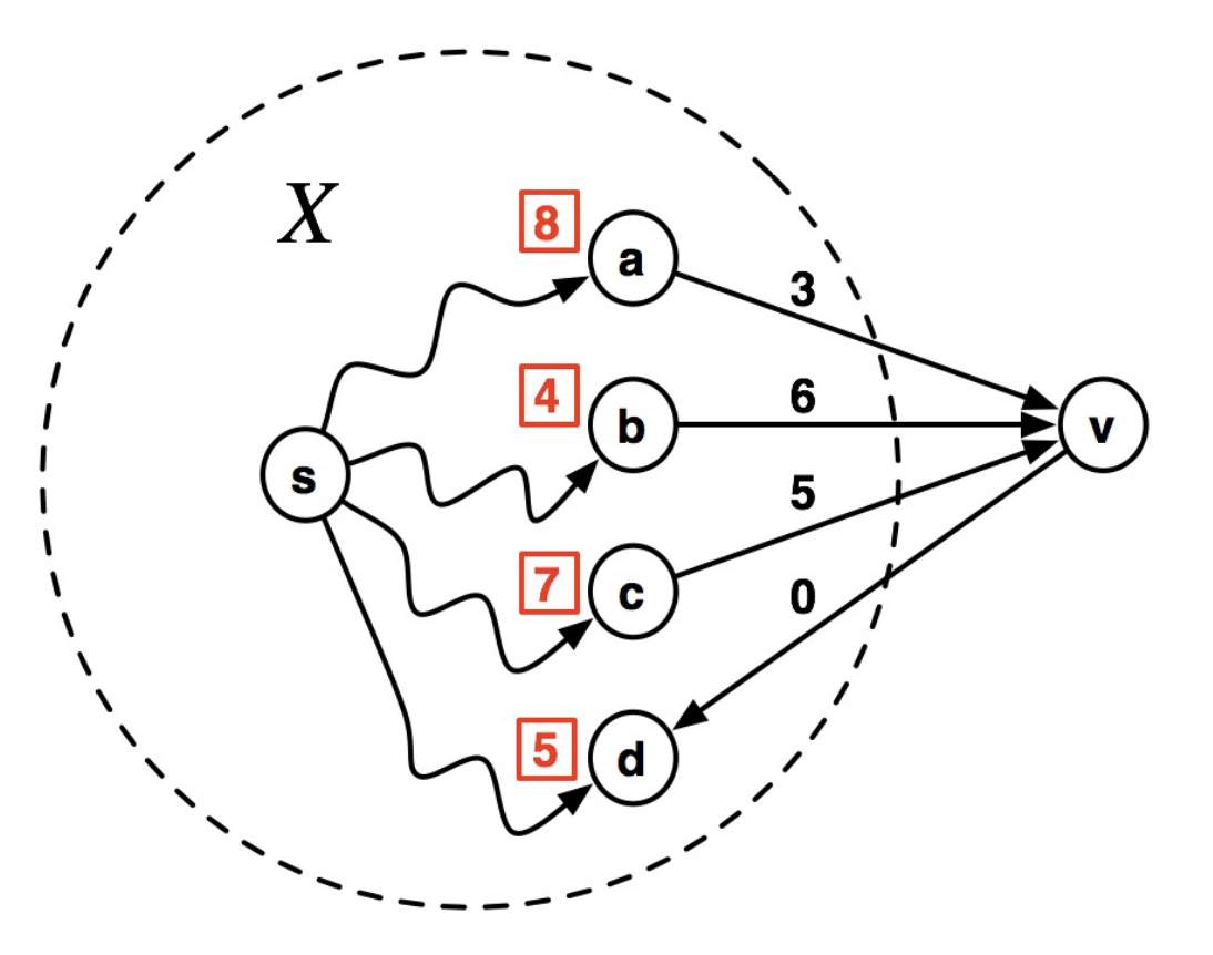
Suppose that an oracle has told us the shortest paths from $s$ to all vertices except for the vertex $v$, shown in red squares. How can we find the shortest path to $v$?

Let $\delta_G(i,j)$ be the weight of shortest path from $i$ to $j$ in graph $G$. Then:

$$ \begin{align} \delta_G(s,v) = \min(&\delta_G(s,a)+3,\\ &\delta_G(s,b)+6,\\ &\delta_G(s,c)+5 ) \end{align} $$

sub-paths property

any sub-path of a shortest path is itself a shortest path.

The sub-paths property makes it possible to construct shortest paths from smaller shortest paths.

If a shortest path from New Orleans to Boston goes through Atlanta, then that path is built from shortest path from New Orleans to Atlanta, and from Atlanta to Boston.

Dijkstra's property

Suppose we have a set of vertices $X$ whose shortest paths are known. Can we efficiently determine the shortest path to any of the vertices in its frontier?

For any partitioning of vertices $V$ into

• $X$
  • The set of vertices we know the shortest paths to
• $Y = V \setminus X$
  • everything else

Given a source vertex $s \in X$, by the sub-paths property:

$$p(v,x) = \min_{x \in X} (\delta_G(s,x) + w(x,v))$$

This is the shortest path to frontier vertex $v$ through $x$.

$$p(y) = \min_{y \in Y} p(y) = \min_{y \in Y} \delta_G(s, y)$$

$y$ is the frontier vertex closest to the source $s$. This is the shortest path distance to $y$ from $s$.

We can use this property to iteratively add vertices to our set of "known vertices"

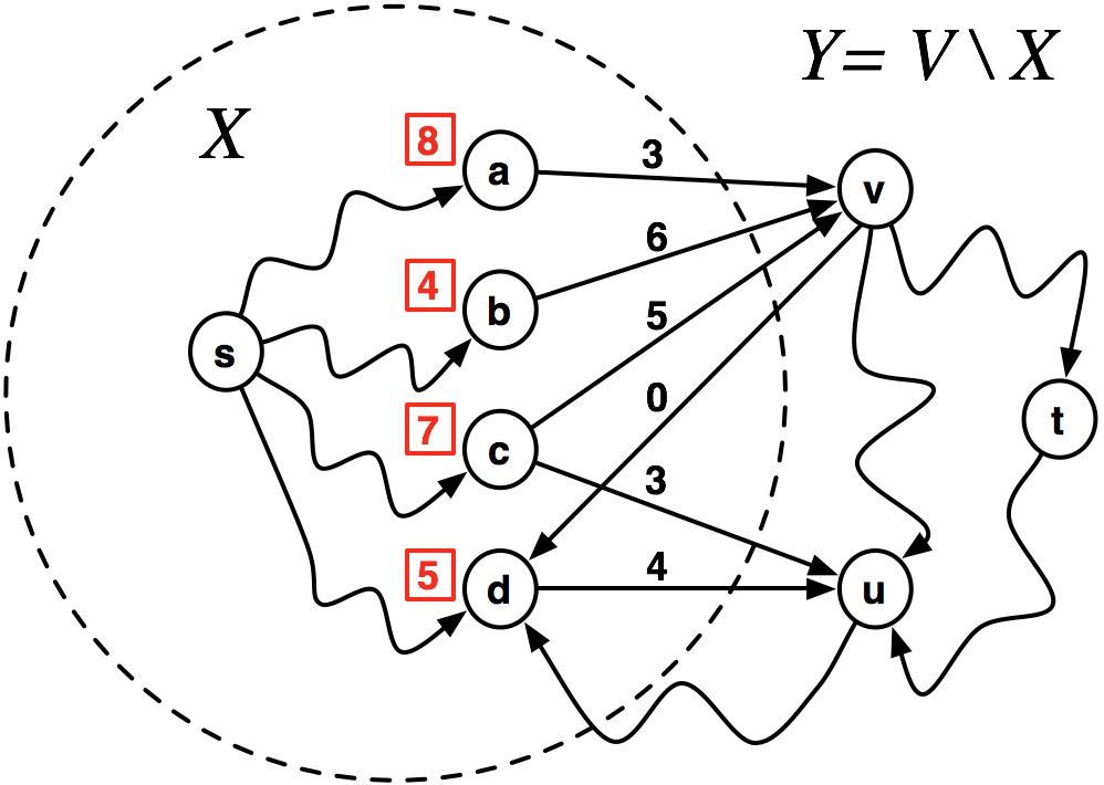
Which vertex will be added to $X$ next?

By going through vertex $d$, a path exists to get to $u$ with a cost of $9$.

$~~~~~\delta_G(s,u) = \delta_G(s,d) + w(d,u) = 5 + 4 = 9$

The shortest path to vertex $v$ is through $b$ with a cost of 10.

$~~~~~\delta_G(s,v) = \delta_G(s,b) + w(b,v) = 4 + 6 = 10$

Full details

$$ \begin{align} \delta_G(s,v) = \min(&\delta_G(s,a) + w(a,v) = 8 + 3 = 11,\\ &\pmb{\delta_G(s,b) + w(b,v) = 4 + 6 = 10}, \\ &\delta_G(s,c) + w(c,v) = 7 + 5 = 12 \\ \end{align} $$$$ \begin{align} \delta_G(s,u) = \min(&\delta_G(s,c) + w(c,u) = 7 + 3 = 10, \\ &\pmb{\delta_G(s,d) + w(d,u) = 5 + 4 = 9} ) \end{align} $$

$\texttt{Vertex } \pmb{u}$ will be added to the known set of vertices next.

Iteratively expanding our known vertices

The sub-paths property suggests that we can continue to expand the set of our "known" vertices by identifing and adding the the frontier vertex the shortest distance from $s$.

This will ensure that we visit nodes in an order to identify actual shortest paths.

By visiting nodes in order of increasing distance from the source, we will find the shortest path from $a \rightarrow c$.

Dijkstra's Algorithm

The final algorithm can be viewed as an instance of priority-first search, using the path length as the priority criterion.

1. Initialize frontier to $(s, 0)$
2. While frontier not empty:
   • pop from the frontier the minimum node $\pmb{v}$ with distance $\pmb{d}$ from the source.
   • set $\texttt{result}(v) = d$
     • this is the weight of the shortest path from $\pmb{s}$ to $\pmb{v}$
   • For each neighbor $\pmb{n}$ of $\pmb{v}$ with edge weight $\pmb{w}$, add $\pmb{n}$ to frontier with distance $\pmb{d} + \pmb{w}$
3. return $\texttt{result}$

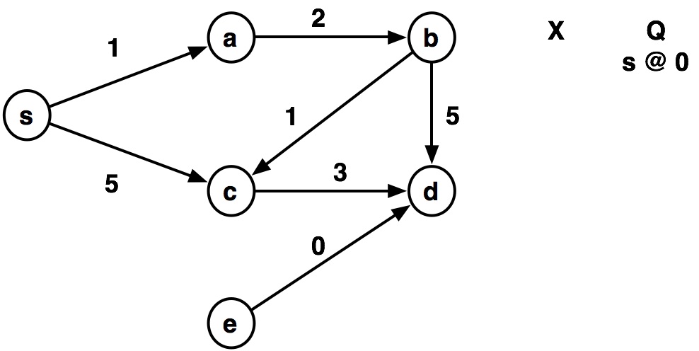
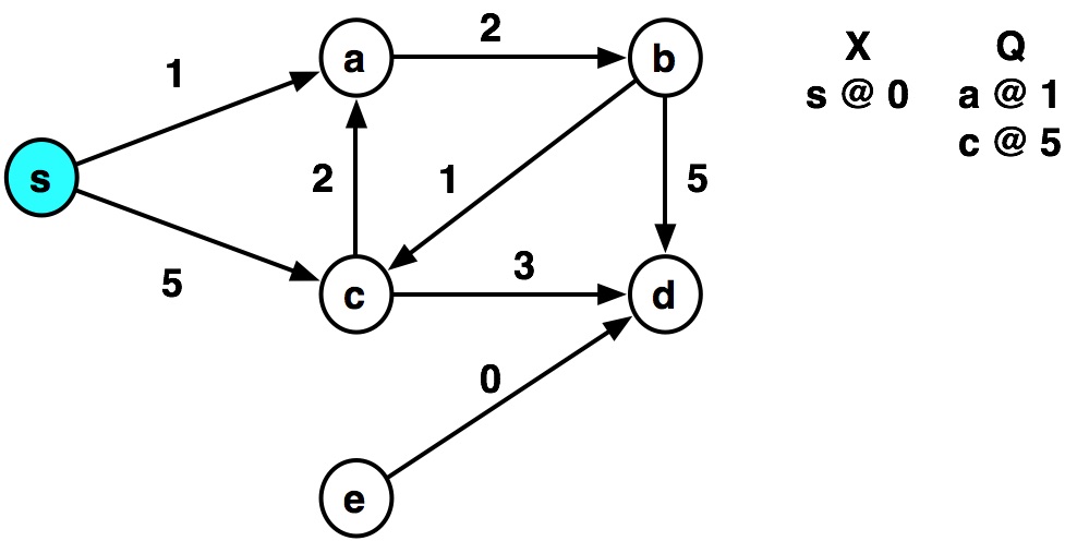
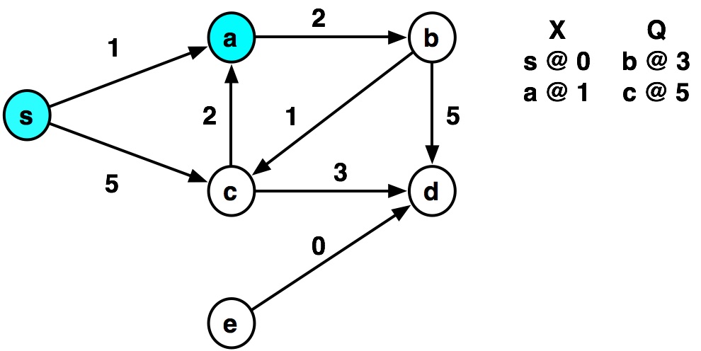
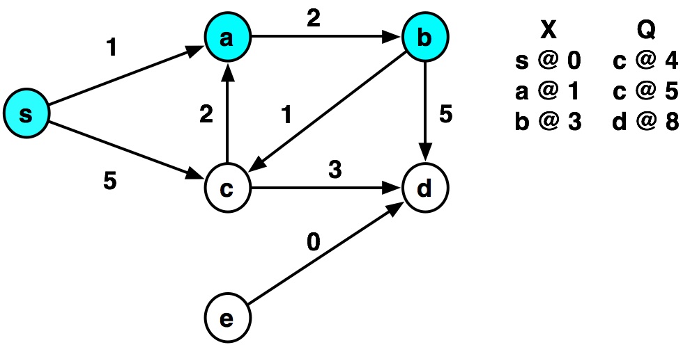
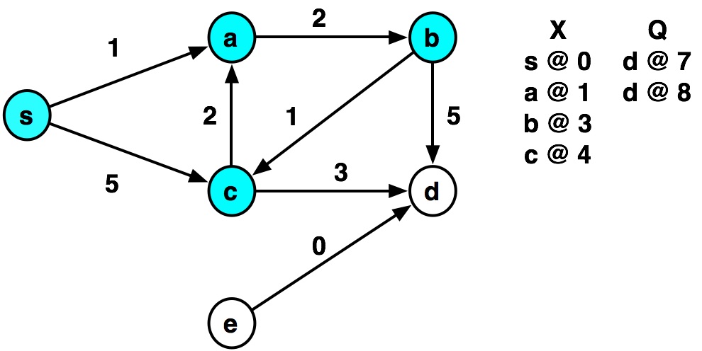
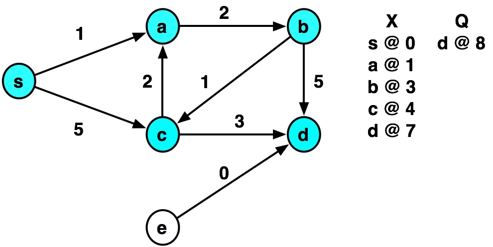
Example by hand

def dijkstra(graph, source):
    def dijkstra_helper(visited, frontier):
        if len(frontier) == 0:
            return visited
        else:
            # Pick next closest node from heap
            distance, node = heappop(frontier)
            print('visiting', node)
            if node in visited:
                # Already visited, so ignore this longer path
                return dijkstra_helper(visited, frontier)
            else:
                # We now know the shortest path from source to node.
                # insert into visited dict.
                visited[node] = distance
                print('...distance=', distance)
                # Visit each neighbor of node and insert into heap.
                # We may add same node more than once, heap
                # will keep shortest distance prioritized.
                for neighbor, weight in graph[node]:
                    heappush(frontier, (distance + weight, neighbor))                
                return dijkstra_helper(visited, frontier)
        
    frontier = []
    heappush(frontier, (0, source))
    visited = dict()  # store the final shortest paths for each node.
    return dijkstra_helper(visited, frontier)

graph = {
            's': {('a', 1), ('c', 5)},
            'a': {('b', 2)},
            'b': {('c', 1), ('d', 5)}, 
            'c': {('a', 2), ('d', 3)},
            'd': {},
            'e': {('d', 0)}
        }
        

dijkstra(graph, 's')

visiting s
...distance= 0
visiting a
...distance= 1
visiting b
...distance= 3
visiting c
...distance= 4
visiting c
visiting a
visiting d
...distance= 7
visiting d

{'s': 0, 'a': 1, 'b': 3, 'c': 4, 'd': 7}

Correctness of Dijkstra's Algorithm

The algorithm maintains an invariant that each visited element $x \in X$ contains the shortest path from $s$ to $x$.

• That is, visited[x] $=\delta_G(s,x)$

• We know this is true after visiting the source, since $\delta_G(s,x)=$ visited[x] $=0$
• Dijkstra's property ensures that each element we remove from the heap also maintains this property

Work of Dijkstra's Algorithm

The two key lines are:

distance, node = heappop(frontier)

and

for neighbor, weight in graph[node]:
    heappush(frontier, (distance + weight, neighbor))

What is work and span of heappop and heappush?

$O(\lg n)$ work and span for each, for a heap of size $n$.

How many times will we call these functions?

Once per edge, since a node may be added to the heap multiple times for each edge.

Total work?

$O(|E| \log |E|)$

Note that we assume constant time dict operations:

• visited[node] = distance
• for neighbor, weight in graph[node]:
• These result in an additional $O(|V| + |E|)$ work, but are dominated by the above.

Because this is a serial algorithm, the span is also $O(|E| \log |E|)$

Potential Optimization

When we visit vertex $b$, we add $c$ to the queue a second time.

Alternatively, we could update the existing value and reheap up or down as necessary.

This would ensure that our heap were never larger than $|V|$, giving us $O(\log |V|)$ heappush and heappop operations rather than $O(\log |E|)$ ones.

With this optimization, we can get a runtime for Dijkstra's of:

$O(|E| \log |V|)$

What is the shortest way to travel from Rotterdam to Groningen, in general: from given city to given city. It is the algorithm for the shortest path, which I designed in about twenty minutes. One morning I was shopping in Amsterdam with my young fiancée, and tired, we sat down on the café terrace to drink a cup of coffee and I was just thinking about whether I could do this, and I then designed the algorithm for the shortest path.

As I said, it was a twenty-minute invention. In fact, it was published in '59, three years later. The publication is still readable, it is, in fact, quite nice. One of the reasons that it is so nice was that I designed it without pencil and paper. I learned later that one of the advantages of designing without pencil and paper is that you are almost forced to avoid all avoidable complexities. Eventually, that algorithm became to my great amazement, one of the cornerstones of my fame.

— Edsger Dijkstra, in an interview with Philip L. Frana, Communications of the ACM, 2001