Agenda:
- "Dynamic Programming" Paradigm
So far, we've looked at 3 different paradigms of algorithm design:
- Divide and Conquer
- Brute Force
- Greedy
(Randomization can be added to any of these.)
Divide and Conquer and Greedy both had a restriction to them in that we always recurse on one or more solutions to fixed size subproblems.
In certain cases, for example using a greedy approach for the Knapsack Problem, this prevented us from reaching an optimal solution.
What if we generalized our approach to consider all possible subproblems? This is sort of a hybrid of brute force and Greedy/Divide and Conquer.
0-1 Knapsack
Suppose there are $n$ objects, each with a value $v_i$ and weight $w_i$. You have a "knapsack" of capacity $W$ and want to fill it with a set of objects $X \subseteq [n]$ so that $w(X) \leq W$ and $v(X)$ is maximized.
We saw previously that a greedy approach works only if we're allowed to take fractional parts of the objects. The problem was that a greedy approach didn't really take leftover capacity into account.
Recall that for greedy algorithms to be correct, we needed to prove that the greedy choice combined with an optimal solution for a smaller subproblem was also optimal (the optimal substructure property).
Fractional Knapsack had this property, but 0-1 Knapsack did not. Why?
We can give a simple counterexample with 2 objects that have weights/values $(10, 5), (9, 3)$ with $W=5.$
| index | value | weight |
|---|---|---|
| 0 | 10 | 5 |
| 1 | 9 | 3 |
The problem is that the greedy choice to maximize value/weight is incorrect because we can have leftover capacity. We really need to look at all possible choices of objects and their associated optimal solutions.
Exploring Multiple Solutions
| index | value | weight |
|---|---|---|
| 0 | 10 | 5 |
| 1 | 9 | 3 |
Let $OPT(n, W)$ be an optimal solution to the Knapsack problem for a set of objects $S$ where we are choosing the object at index $n$ and we have a current capacity of $W$.
Now, we can make the following simple observation:
If object $n$ is in the optimal solution, then
$OPT(n, W)= \{n\} \cup OPT(n-1, W-w(n)).$
else
$OPT(n, W) = OPT(n-1, W)$.
Optimal Substructure for Knapsack
For any set $S$ of $n$ objects and $W>0$, we have
$\begin{align} v(OPT(n, W)) = \max \{&v(n) + v(OPT(n-1, W - w(n))), \\ &v(OPT(n-1, W))\} \end{align}$
with respect to choosing some object $n$.
In a way, this really isn't saying much. Put plainly we're just saying that the optimal solution either contains object $n$ or it doesn't.
Note that our optimal substructure recurrence depends both on the number of objects as well as their weights.
From our example:
| index | value | weight |
|---|---|---|
| 0 | 10 | 5 |
| 1 | 9 | 3 |
For choosing object $1$, we have that:
$\begin{align} v(OPT(1, 5)) &=& \max\{v(1) + v(OPT(0, 2)), v(OPT(0, 5))\} \\ &=& \max\{9, 10\} \\ &=& 10. \\ \end{align}$
Does this give us an algorithm?
The recurrence
$\begin{align} v(OPT(n, W)) = \max \{&v(n) + v(OPT(n-1, W - w(n))), \\ &v(OPT(n-1, W))\} \end{align}$
The number of recursive calls doubles in every recursion. But suppose all items have weight 1, is there a glaring inefficiency we can fix? Let's consider the recursion tree:
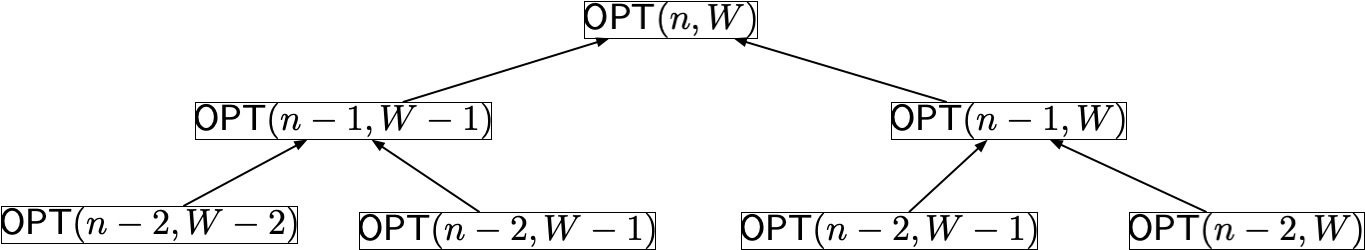
If we blindly recompute the redundant calls when they are encountered, then we will do $\Omega(2^n)$ work and $O(n)$ span even if we can take all the items.
However, suppose that whenever we need to compute $v(OPT(i, w)$, we compute it once and save the result for later use (e.g., in a suitable data structure) -- this is called memoization. Then, we no longer have a binary tree but rather a directed acyclic graph or DAG.
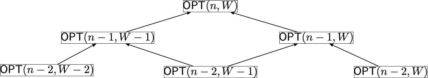
The number of nodes in this DAG will allow us to determine the work of this algorithm, and the longest path in the DAG will allow us to determine the span.
Memoization
When performing memoization, we can either proceed top-down or bottom-up:
top-down: use recursion as usual, but maintain a hashmap or related data structure to quickly look up solutions previously computed
bottom-up: start with solutions to smallest problem instances, then proceed to larger instances. This is typically implemented by filling a table.
Bottom-up Memoization Example
We can use our recurrence to build and fill in a table.
$\begin{align} v(OPT(n, W)) = \max \{&v(n) + v(OPT(n-1, W - w(n))), \\ &v(OPT(n-1, W))\} \end{align}$
| W |
|||||||
|---|---|---|---|---|---|---|---|
| n |
0 | 1 | 2 | 3 | 4 | 5 | |
| 0 | |||||||
| 1 | |||||||
| 2 | |||||||
| index | value | weight |
|---|---|---|
| 0 | 10 | 5 |
| 1 | 6 | 3 |
| 2 | 7 | 2 |
First we fill in item $0$ by simply considering it. For each capacity, can it fit in a bag of that capacity?
| W |
|||||||
|---|---|---|---|---|---|---|---|
| n |
0 | 1 | 2 | 3 | 4 | 5 | |
| 0 | 0 | 0 | 0 | 0 | 0 | 10 |
|
| 1 | |||||||
| 2 | |||||||
Then we use the recurrence to fill in the following rows.
$\begin{align} v(OPT(n, W)) = \max \{&v(n) + v(OPT(n-1, W - w(n))), \\ &v(OPT(n-1, W))\} \end{align}$
| index | value | weight |
|---|---|---|
| 0 | 10 | 5 |
| 1 | 6 | 3 |
| 2 | 7 | 2 |
| W |
|||||||
|---|---|---|---|---|---|---|---|
| n |
0 | 1 | 2 | 3 | 4 | 5 | |
| 0 | 0 | 0 | 0 | 0 | 0 | 10 |
|
| 1 | 0 | 0 | 0 | 6 | |||
| 2 | |||||||
$\begin{align} v(OPT(1, 3)) = \max \{6 + &v(OPT(0, 3-3)),\\ &v(OPT(0, 3)) \} \end{align}$
| index | value | weight |
|---|---|---|
| 0 | 10 | 5 |
| 1 | 6 | 3 |
| 2 | 7 | 2 |
| W |
|||||||
|---|---|---|---|---|---|---|---|
| n |
0 | 1 | 2 | 3 | 4 | 5 | |
| 0 | 0 | 0 | 0 | 0 | 0 | 10 |
|
| 1 | 0 | 0 | 0 | 6 | 6 | 10 | |
| 2 | |||||||
$\begin{align} v(OPT(1, 5)) = \max \{6 + &v(OPT(0, 5-3)),\\ &v(OPT(0, 5)) \} \end{align}$
$\begin{align} v(OPT(1, 5)) = \max \{6 + 0, 10 \} = 10 \end{align}$
| index | value | weight |
|---|---|---|
| 0 | 10 | 5 |
| 1 | 6 | 3 |
| 2 | 7 | 2 |
| W |
|||||||
|---|---|---|---|---|---|---|---|
| n |
0 | 1 | 2 | 3 | 4 | 5 | |
| 0 | 0 | 0 | 0 | 0 | 0 | 10 |
|
| 1 | 0 | 0 | 0 | 6 | 6 | 10 | |
| 2 | 0 | 0 | 7 | 7 | 7 | 13 | |
$\begin{align} v(OPT(2, 5)) = \max \{7 + &v(OPT(1, 5-2)),\\ &v(OPT(1, 5)) \} \end{align}$
$\begin{align} v(OPT(2, 5)) = \max \{7 + 6, 10 \} = 13 \end{align}$
import random

def recursive_knapsack(objects, i, W):
    v, w = objects[i]
    if (i == 0):
        if (w <= W):
            return(v)
        else:
            return(0)
    else:
        if (w <= W):
            take = v + recursive_knapsack(objects, i-1, max(W-w, 0))
            dont_take = recursive_knapsack(objects, i-1, W)
            return(max(take, dont_take))
        elif (W == 0):
            return(0)
        else:
            return(recursive_knapsack(objects, i-1, W))
def tabular_knapsack(objects, W):
    n = len(objects)
    # we'll rely on indices to also represent weights, so we'll index from 1...W
    # in the weight dimension of the table
    OPT = [[0]*(W+1)]

    # initialize the first row of the table
    for w in range(W+1):
        if (objects[0][1] <= w):
            OPT[0][w] = objects[0][0]
        else:
            OPT[0][w] = 0

    # use the optimal substructure property to compute increasingly larger solutions
    for i in range(1,n):
        OPT.append([0]*(W+1))
        v_i, w_i = objects[i]
        for w in range(W+1):
            if (w_i <= w):
                OPT[i][w] = max(v_i + OPT[i-1][w-w_i], OPT[i-1][w])
            else:
                OPT[i][w] = OPT[i-1][w]

    print(OPT)
    return(OPT[n-1][W])

W = 5
objects = [(10,5), (6,3), (7,2)]
print(tabular_knapsack(objects, W))
[[0, 0, 0, 0, 0, 10], [0, 0, 0, 6, 6, 10], [0, 0, 7, 7, 7, 13]]
13
Elements of Dynamic Programming
This is what we call dynamic programming. The elements of a dynamic programming algorithm are:
- Optimal Substructure
- Recursion DAG
The correctness of the dynamic programming approach follows from the optimal substructure property (i.e., induction). If we can prove that the optimal substructure property holds, and that we compute a solution by correctly implementing this property then our solution is optimal.
As with divide and conquer algorithms, achieving a good work/span can be tricky. We can minimize redundant computation by memoizing solutions to all subproblems, which we can do:
top-down by saving the result of a recursive call the first time we encounter it.
bottom-up by filling in a table using the recurrence as a guide.
Work and Span in Dynamic Programming
Since we memoize the solution to every distinct subproblem, the number of nodes in the DAG is equal to the number of distinct subproblems considered, that is, the number of cells in the table..
There are at most $O(nW)$ nodes in the table, and the longest path in the DAG is $O(n)$.
The longest path in the DAG represents the span of our dynamic programming algorithm.
Each node requires $O(1)$ work/span, so the work is $O(nW)$ and the span is $O(n)$.
Why "Dynamic Programming"?
The mathematician Richard Bellman coined the term "dynamic programming" to describe the recursive approach we just showed. The optimal substructure property is sometimes referred to as a "Bellman equation." But why did he call it dynamic programming?
There is some folklore around the exact reason. But it could possibly be because "dynamic" is a really dramatic way to describe the search weaving through the DAG. The term "programming" was used in the field of optimization in the 1950s to describe an optimization approach (e.g., linear programming, quadratic programming, mathematical programming).