So far we have focused on the basic environment for designing algorithms:
- Model of computation (Work/Span)
- Algorithm specification language (SPARC)
- Asymptotic analysis of performance (Recurrences)
- Abstract Data Types (sequences)
We will now shift our focus to algorithmic paradigms and see examples of how they work in different problem areas.
First we will look at how problems can be related to one another through reductions and then define the concept of a search space for an problem.
Reductions
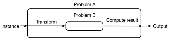
We say that a problem $A$ is reducable to a problem $B$ if an instance of problem $A$ can be turned into some instance of $B$. So, this means we can solve problem $A$ using these three steps:
The input $\mathcal{I}_A$ to $A$ is transformed into one or more instances of $B$
Solve these instances of $B$.
Use these output(s) to construct the solution to $\mathcal{I}_A$.
It's convenient to view this schematically as:
What is the running time of our generic algorithm for solving $A$?
The time to solve $A$ on an input $\mathcal{I}_A$:
- the time to construct one or more instances of $B$
- the time to solve one or more instances of $B$
- the time to construct the solution to $\mathcal{I}_A$
We say that a reduction is efficient if the running time of the input/output transformations do not exceed the running time of the problem being solved.
Example: Reduce min to sorting
# reduction from min-finding to sorting.
def my_min(L):
    return sorted(L)[0]

my_min([1, 2, 3, 99, 5, 6, 7, -1])
-1
In this reduction, the input transformation is trivial, we sort the list, and the output transformation consists of taking the first element of the sorted list.
What about in the other direction, is selection_sort an example of reducing sorting to min?
def selection_sort(L):
    for i in range(len(L)):
        m = L.index(min(L[i:]))
        L[i], L[m] = L[m], L[i]
    return L

selection_sort([2, 1, 4, 3, 9, -1, -2])
[-2, -1, 1, 2, 3, 4, 9]
This is not really a reduction - selection_sort depends on a bunch of successive calls to min.
Relationship between problems $A$ and $B$
If we construct a valid reduction from $A$ to $B$, then we have shown that problem $A$ is "no harder" than $B$. If $A$ were strictly harder than $B$, we couldn't solve $A$ with a reduction to $B$!
Suppose we are speculating about the difficulty of a scary looking problem $A$. Now suppose we manage to find a problem $B$ so that we have an efficient reduction from $A$ to $B$.
The runtime (work or span) of $A$ is upper bounded by the runtime of any algorithm for $B$, without having found an algorithm for $A$ or $B$!
This a useful concept that is used to "map" the complexity of problems, whether or not we have efficient algorithms! (We'll get to this in more detail at the end of the semester.)
Reductions Key Points
If $A$ is reducible to $B$ then:
- $A$ is not harder than $B$
- $B$ is at least as hard as $A$
So, by reducing min to sort, we've just shown that
minis no harder thansortsortis at least as hard asmin.
More Reductions
Median Finding: Find the median of an unsorted list $L$ of length $n$.
Reduction: No input transformation, just sort $L$ and take the element at position $\lfloor n/2 \rfloor$.
This shows finding the median of a list is no harder than sorting the list. What can we conclude about finding the median (i.e., selection)?
Upper bound?
$O(n\log n)$, since this is the best runtime for sorting.
It turns out that there is an $O(n)$ algorithm for median finding. What does this say about the best possible runtime for sorting?
$\Omega(n)$, since this is the best runtime for median finding.
What about the more general problem of finding the $k^\texttt{th}$ smallest number in a list of length $n$?
median finding is reducible to find the kth smallest number in a list
The kth smallest number problem is atleast as hard as median.
The runtime of kth smallest number is $\Omega(n)$.
Example: Convex Hull:
Given a set of points in the plane, find the extreme points and return them in counterclockwise order. This generates the "convex hull" of the point set.
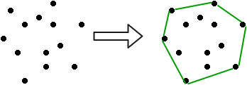
The extreme points always create a convex boundary around the point set, hence the name.
How difficult is convex hull, relative to other computational problems?
It turns out that we can reduce from sorting to convex hull.
That means that interestingly, convex hull is at least as hard as sorting!
Reduction: Sorting -> Convex Hull:
Given a list of length $n$ to sort, we can construct a point set by taking each list element $a\in L[i]$ and creating a corresponding point $(a, a^2)$.
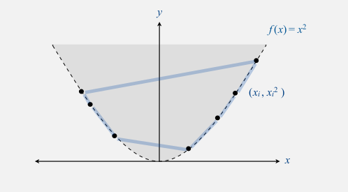
Any algorithm that returns the points of the convex hull of this point set in counterclockwise order will produce the elements of the original list in sorted order.
Can we say anything else? Well, it turns out sorting is $\Omega(n \log n)$. So computing the convex hull is $\Omega(n \log n)$, otherwise we could do better than $O(n \log n)$ for sorting a list.
Search Spaces and Brute-Force
Let's now focus on another way to think about the difficulty of a computational problem, which motivates a very simple algorithmic paradigm.
As the name suggests, the "brute force" paradigm for an instance $\mathcal{I}_A$ of problem $A$ just looks at every possible solution and checks each one.
Brute Force Sorting
Let's consider the problem of sorting by brute force. Given a list $L$ of length $n$, how would this work?
We'd need to consider every possible sorted order of length $n$ on the elements in $L$. How many are there?
$n!$ - why?
Now, if we can explicitly generate all permutations, we'd need to check each one for "sortedness". How long does that take?
Thus, sorting by brute force takes $O(n \cdot n!)$ work. For $n=100$, this is at least $10^{100}$!!
There are only about $10^{80}$ atoms in the known universe...
This is horribly inefficient.
Is there any upside to brute force?
The work of this algorithm for sorting is astronomical (literally), but let us consider the span.
Span
How quickly can we check (in parallel) that a list is sorted?
For all $i=0,\ldots,n-2$, check that $L[i] \leq L[i+1]$.
This can be done with a parallel filter.
Then, do a parallel reduce to check that all $n-1$ inequalities are met in $O(\log n)$ span.
Overall it takes $O(\log n)$ span to check that a list is sorted, for each candidate permutation. All permutations can be checked concurrently.
So, while brute force sorting is not at all work-efficient, we can achieve a very efficient span!
Brute Force Maximum
Consider the problem of finding the maximum element in a list $L$ of length $n$.
What is the search space?
Since the maximum of a list is just an element in the list, the search space is all $n$ elements in the list.
How do we check whether each candidate solution is the correct one?
If each candidate $x$ is greater than or equal to every other $y\in L$, then $x$ is the solution.
This takes $O(n)$ work.
Over all $n$ elements, the brute force approach takes $O(n^2)$ work and and $O(\log n)$ span (why?).
How does this compare to other approaches we've seen?
Using iterate: $O(n)$ work, $O(n)$ span
Using reduce: $O(n)$ work, $O(\log n)$ span
Brute-force: $O(n^2)$ work, $O(\log n)$ span
Why Discuss Brute Force?
It gives us an upper bound on the potential runtime
It is a useful theoretical idea
- We will revisit it when thinking about complexity classes
Bruce Force algorithms are simple
- Sometimes, it is convenient to prototype a brute force solution first before implementing a more complex and efficient one.