Agenda:
- Different ways to model computational cost
- Random Access Machine
- Language Based Models
- SPARC's Cost Model
Recall first lecture:
def linear_search(mylist, key):        #   cost         number of times run
    for i,v in enumerate(mylist):      #   c1               n
        if v == key:                   #   c2               n
            return i                   #   c3               0
    return -1                          #   c4               1
$\hbox{Cost(linear-search, } n) = c_1n + c_2n + c_4 = O(n)$
machine-based cost model
- define the cost of each instruction
- runtime is sum of costs of each instruction
Random Access Machine model
- "Simple" operations (+, *, =, if) take exactly one time step
- no matter the size of operands
- loops consist of many single-step operations
- memory access takes one step
- unbounded memory
- each cell holds integers of unbounded size
- assumes sequential execution
- one input tape, one output tape
Hypothetically, we could compute the run time of an algorithm:
- compute the number of steps
- determine the number of steps per second our machine can perform
- time = steps / steps per second
All models make incorrect assumptions. What are some that the RAM model makes?
- multiplication does not take the same time as addition
- cache is faster than RAM
Not terrible assumptions since we are interested in asymptotic analysis.
E.g., if cache lookup is half the time of RAM lookup, then we're "only" off by a factor of 2.
E.g. $2n \in O(n)$
Language Based Cost Models
- Define a language to specify algorithms
- Assign a cost to each expression
- Cost of algorithm is sum of costs for each expression
Work-Span model
- We can define this model for SPARC
Recall our definitions of work and span
work: total number of primitive operations performed by an algorithm
span: longest sequence of dependent operations in computation
- also called: critical path length or computational depth
intuition:
work: total operations required by a computation
span: minimum possible time that the computation requires, measure of how parallelized and algorithm is
For a given SPARC expression $e$, we will analyze the work $W(e)$ and span $S(e)$
Composition
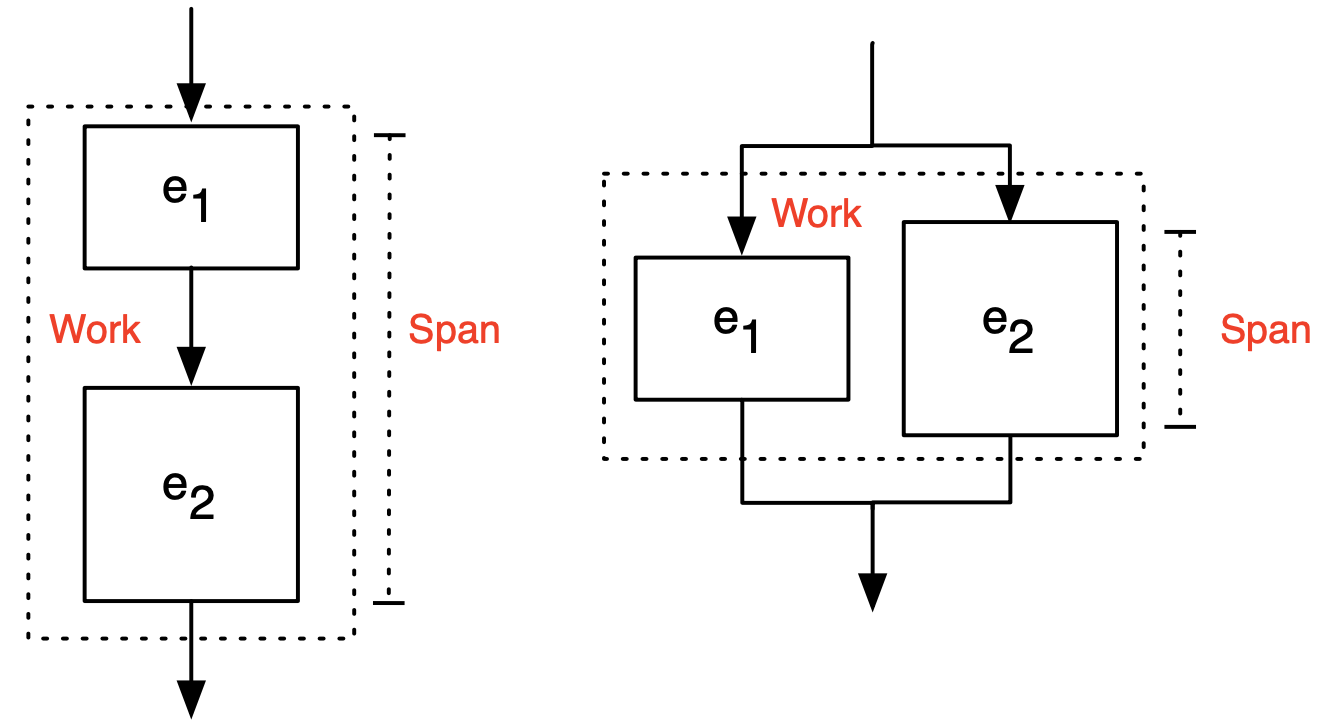
$(e_1, e_2)$: Sequential Composition
- Work and span are both sum of both expression
- Work == Span
$(e_1 || e_2)$: Parallel Composition
- Work is the sum of both expresions
- Span is the max of the two
Rules of composition
| $\mathbf{e}$ | $\mathbf{W(e)}$ | $\mathbf{S(e)}$ |
|---|---|---|
| $v$ | $1$ | $1$ |
| $\mathtt{lambda}\:p\:.\:e$ | $1$ | $1$ |
| $(e_1, e_2)$ | $1 + W(e_1) + W(e_2)$ | $1 + S(e_1) + S(e_2)$ |
| $(e_1 || e_2)$ | $1 + W(e_1) + W(e_2)$ | $1 + \max(S(e_1), S(e_2))$ |
| $(e_1 e_2)$ | $W(e_1) + W(e_2) + W([\hbox{Eval}(e_2)/x]e_1) + 1$ | $S(e_1) + S(e_2) + S([\hbox{Eval}(e_2)/x]e_1) + 1$ |
let val $x=e_1$ in $e_2$ end |
$1 + W(e_1) + W([\hbox{Eval}(e_1)/x]e_2)$ | $1 + S(e_1) + S([\hbox{Eval}(e_1)/x]e_2)$ |
| $\{f(x)\mid x\in A\}$ | $1+\sum_{x\in A} W(f(x))$ | $1+\max_{x\in A} S(f(x))$ |
Sequential composition: $e_1, e_2$
$W(e_1, e_2) = 1 + W(e_1) + W(e_2)$
$S(e_1, e_2) = 1 + S(e_1) + S(e_2)$
Parallel composition: $e_1 || e_2$
$W(e_1 || e_2) = 1 + W(e_1) + W(e_2)$
$S(e_1 || e_2) = 1 + \max(S(e_1), S(e_2))$
We are making a couple of assumptions about $e_1$ and $e_2$.
In a pure functional language, we can run two functions in parallel if there is no explicit sequencing.
- no side effects
- data persistence
function application: $e_1 e_2$
Apply $e_1$ using as input the result of $e_2$
e.g,
$\mathtt{lambda} (\: x \: . ~ x * x)(6/3)$
$W(e_1 e_2) = W(e_1) + W(e_2) + W([\hbox{Eval}(e_2)/x]e_1) + 1$
- $\hbox{Eval}(e)$ evaluates to be the return of expression $e$
- $[v/x]e$: replace all free (unbound) occurrences of $x$ in $e$ with value $v$
- e.g., $[10/x](x^2+10) \rightarrow 110$
- $W([\hbox{Eval}(e_2)/x]e_1)$ is the cost of substituting the output of $e_2$ into all instances of $x$ in $e_1$
We won't get into the weeds of calculating $W([\hbox{Eval}(e_2)/x]e_1)$ in this course.
We can simplify:
$W(e_1 e_2) = W(e_1) + W(e_2)$
$S(e_1 e_2) = S(e_1) + S(e_2)$
Parallelism, revisited
how many processors can we use efficiently?
average parallelism:
$$ \overline{P} = \frac{W}{S} $$
To increase parallelism, we can
- decrease span
- increase work (but that's not really desireable, since we want the overall cost to be low)
work efficiency: a parallel algorithm is work efficient if it performs asymptotically the same work as the best known sequential algorithm for the problem.
So, we want a work efficient parallel algorithm with low span.
Coming up
We will introduce a fundamental tool in the analysis of algorithms: recurrences.